Package bdvis: Biodiversity data visualizations using R is helpful to understand completeness of biodiversity inventory, extent of geographical, taxonomic and temporal coverage, gaps and biases in data. Package bdvis version 0.2.6 is on CRAN now. This version has several features added since version 0.1.0. I plan to post set of blog entries here to describe some of the key features of the package with some code snippets.
The function bdcomplete computes completeness values for each cell. So after dividing the extent of the dataset in cells (via the getcellid function), this function calculates the Chao2 estimator of species richness. In simple terms, the function estimates looking at the data records in each cell and how many species are represented, how complete that dataset.
The following code snippet shows how the data downloaded from Global Biodiversity Information Facility GBIF Data Portal. The .zip file downloaded using the portal has a file occurrence.txt which contains the data records. Copy that file in the working folder and try the following script.
library(bdvis)

# Download GBIF data from data.gbif,org portal and
# extract occurrence.txt file in Data folder
occurrence <- read.delim( 'occurrence.txt',
                         quote='', stringsAsFactors=FALSE)
# Set configuration variables to format data
conf <- list(Latitude='decimalLatitude',
             Longitude='decimalLongitude',
             Date_collected='eventDate',
             Scientific_name='specificEpithet')
occurrence <- format_bdvis(occurrence, config=conf)
# Compute completeness and visualize using mapgrid
comp=bdcomplete(occurrence)
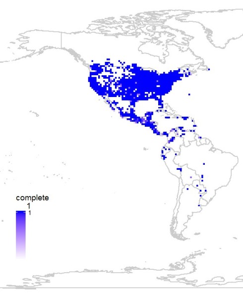
mapgrid(comp,ptype='complete')
The completeness function produces a graph showing Completeness vs number of Species. More points in higher range of completeness indices indicates better data.
Now to visualize the data spatially, if any particular region needs better sampling the function mapgrid can now be used with ptype = “complete” parameter. This plots all the grids that have data records more than recs parameter (default = 50) using a color range from light purple to dark blue. Darker the color better the data in that cell.
References:
- Barve, V., & Otegui, J. (2016). bdvis: visualizing biodiversity data in R. Bioinformatics. doi:10.1093/bioinformatics/btw333 Available from
- Barve, V., & Otegui, J. (2016). bdvis: Biodiversity data visualizations Version: 0.2.6 Accessed from https://cran.r-project.org/web/packages/bdvis/index.html


Congrats Vijay! Great and very useful work! I have one doubt. In your bdcomplete function, I noticed that you use an extra parameter (m) for estimating Chao2. This parameter seems to be related to “Date_Collected”. Can you explain me why is this necessary?
Also, I wanted to ask you if you have thought/implemented a similar approach but for comparing different sites/cells via species accumulation/rarefaction curves?
Thanks! Say hi to the family!
Thanks @Fabricio.
If I remember correctly m-1/m is for bias correction. But I will have to look it up. It has been some time since I programmed this function.
Hi Fabricio,
probably you can try with vegan for rarefraction… I did a little function for that. I hope that it is helpful for you
RarefraccionCC <- function(Tabla,factor){
require(vegan)
Tabla1 <- data.frame(Tabla, row.names=factor)
#Tabla1 <- decostand(Tabla1, "pa")
raremax <- min(rowSums(Tabla1))
col1 <- seq(1:nrow(Tabla1)) #Para poner color a las lineas
lty1 <- c("solid","dashed","longdash","dotdash")
rarecurve(Tabla1, sample = raremax, col = "black", lty=lty1, cex = 0.6)
#Para calcular el numero de especies de acuerdo a rarefraccion
UUU <- rarefy(Tabla1, raremax)
print(UUU)
}
Thanks, Alex! I’ll take a look. Gracias!