Tag Archives: maps

India has 100k records on iNaturalist

22 Apr

Biodiversity citizen scientists use iNaturalist to post their observations with photographs. The observations are then curated there by crowd-sourcing the identifications and other trait related aspects too. The data once converted to “research grade” is passed on to GBIF as occurrence records.

Exciting news from India in 3rd week of April 2019 is:

Being interested in biodiversity data visualizations and completeness, I was waiting for 100k records to explore the data. Here is what I did and found out.

Step 1: Download the data from iNaturalist website. Which can be done very easily by visiting the website and choosing the right options.

https://www.inaturalist.org/observations?place_id=6681

I downloaded the file as .zip and extracted the observations-xxxx.csv. [In my case it was observations-51008.csv].

Step 2: Read the data file in R

library(readr)
observations_51008 <- read_csv("input/observations-51008.csv")

Step 3: Clean up the data and set it up to be used in package bdvis.

library(bdvis)

inatc <- list(
  Latitude="latitude",
  Longitude="longitude",
  Date_collected="observed_on",
  Scientific_name="scientific_name"
)

inat <- format_bdvis(observations_51008,config = inatc)

Step 4: We still need to rename some more columns for ease in visualizations like rather than ‘taxon_family_name’ it will be easy to have field called ‘Family’

rename_column <- function(dat,old,new){
  if(old %in% colnames(dat)){
    colnames(dat)[which(names(dat) == old)] <- new
  } else {
    print(paste("Error: Fieldname not found...",old))
  }
  return(dat)
}

inat <- rename_column(inat,'taxon_kingdom_name','Kingdom')
inat <- rename_column(inat,'taxon_phylum_name','Phylum')
inat <- rename_column(inat,'taxon_class_name','Class')
inat <- rename_column(inat,'taxon_order_name','Order_')
inat <- rename_column(inat,'taxon_family_name','Family')
inat <- rename_column(inat,'taxon_genus_name','Genus')

# Remove records excess of 100k
inat <- inat[1:100000,]

Step 5: Make sure the data is loaded properly

bdsummary(inat)

will produce some like this:

Total no of records = 100000 

 Temporal coverage...
 Date range of the records from  1898-01-01  to  2019-04-19 

 Taxonomic coverage...
 No of Families :  1345
 No of Genus :  5638
 No of Species :  13377 

 Spatial coverage ...
 Bounding box of records  6.806092 , 68.532  -  35.0614769085 , 97.050133
 Degree celles covered :  336
 % degree cells covered :  39.9524375743163

The data looks good. But we have a small issue, we have some records from year 1898, which might cause trouble with some of our visualizations. So let us drop records before year 2000 for the time being.

inat = inat[which(inat$Date_collected > "2000-01-01"),]

Now we are ready to explore the data. First one I always like to see is geographical coverage of the data. First let us try it at 1 degree (~100km) grid cells. Note here I have Admin2.shp file with India states map.

mapgrid(inat,ptype="records",bbox=c(60,100,5,40),
        shp = "Admin2.shp")

mapgrid1_c

This shows a fairly good geographical coverage of the data at this scale. We have very few degree cells with no data. How about fines scale though? Say at 0.1 degree (~10km) grid. Let us generate that.

mapgrid(inat,ptype="records",bbox=c(60,100,5,40),
        shp = "Admin2.shp",
        gridscale=0.1) 

mapgrid2_c

Now the pattern is clear, where the data is coming from.

To be continued…

References

Mapping Biodiversity data on smaller than one degree scale

23 Feb

Guest Post by Enjie (Jane) LI

I have been using bdvis package (version 0.2.9) to visualize the iNaturalist records of RAScals project (http://www.inaturalist.org/projects/rascals).

Initially, the mapgrid function in the bdvis version 0.2.9 was written to map the number of records, number of species and completeness in a 1-degree cell grid (~111km x 111km resolution).

I applied this function to the RASCals dataset, see the following code. However, the mapping results are not satisfying. The 1 degree cells are too big to reveal the details in the study areas. Also, the raster grid was on top the basemap, which makes it really hard to associate the mapping results with physical locations.

library(rinat)
library(bdvis)

rascals=get_inat_obs_project("rascals")
conf <- list(Latitude="latitude",
             Longitude="longitude",
             Date_collected="Observed.on",
             Scientific_name="Scientific.name")
rascals <- format_bdvis(rascals, config=conf)
## Get rid of a record with weird location log
rascals <- rascals[!(rascals$Id== 4657868),]
rascals <- getcellid(rascals)
rascals <- gettaxo(rascals)
bdsummary(rascals)

a <- mapgrid(indf = rascals, ptype = "records",
             title = "distribution of RASCals records",
             bbox = NA, legscale = 0, collow = "blue",
             colhigh = "red", mapdatabase = "county",
             region = "CA", customize = NULL)

b <- mapgrid(indf = rascals, ptype = "species",
              title = "distribution of species richness of RASCals records",
              bbox = NA, legscale = 0, collow = "blue",
              colhigh = "red", mapdatabase = "county",
              region = "CA", customize = NULL)

rascals01

rascals02

I contacted developers of the package regarding these two issues. They have been very responsive to resolve them. They quickly added the gridscale argument in the mapgrid function. This new argument allows the users to choose scale (0.1 or 1). The default 1-degree cell grid for mapping.

Here are mapping results from using the gridscale argument. Make sure you have bdvis version 0.2.14 or later.

c <- mapgrid(indf = rascals, ptype = "records",
             title = "distribution of RASCals records",
             bbox = NA, legscale = 0, collow = "blue",
             colhigh = "red", mapdatabase = "county",
             region = "CA", customize = NULL,
             gridscale = 0.1)

d <- mapgrid(indf = rascals, ptype = "species",
             title = "distribution of species richness of RASCals records",
             bbox = NA, legscale = 0, collow = "blue",
             colhigh = "red", mapdatabase = "county",
             region = "CA", customize = NULL,
             gridscale = 0.1)

rascals03

rascals04

We can see that the new map with a finer resolution definitely revealed more information within the range of our study area. One more thing to note is that in this version developers have adjusted the basemap to be on top of the raster layer. This has definitely made the map easier to read and reference back to the physical space.

Good job team! Thanks for developing and perfecting the bdvis package.

References

Visualize completeness of biodiversity data

10 Jun Completeness Visualization

Package bdvis: Biodiversity data visualizations using R is helpful to understand completeness of biodiversity inventory, extent of geographical, taxonomic and temporal coverage, gaps and biases in data. Package bdvis version 0.2.6 is on CRAN now. This version has several features added since version 0.1.0. I plan to post set of blog entries here to describe some of the key features of the package with some code snippets.

The function bdcomplete computes completeness values for each cell. So after dividing the extent of the dataset in cells (via the getcellid function), this function calculates the Chao2 estimator of species richness. In simple terms, the function estimates looking at the data records in each cell and how many species are represented, how complete that dataset.

The following code snippet shows how the data downloaded from Global Biodiversity Information Facility GBIF Data Portal. The .zip file downloaded using the portal has a file occurrence.txt which contains the data records. Copy that file in the working folder and try the following script.

library(bdvis)

# Download GBIF data from data.gbif,org portal and
# extract occurrence.txt file in Data folder
occurrence &lt;- read.delim( 'occurrence.txt',
                         quote='', stringsAsFactors=FALSE)
# Set configuration variables to format data
conf &lt;- list(Latitude='decimalLatitude',
             Longitude='decimalLongitude',
             Date_collected='eventDate',
             Scientific_name='specificEpithet')
occurrence &lt;- format_bdvis(occurrence, config=conf)
# Compute completeness and visualize using mapgrid
comp=bdcomplete(occurrence)
mapgrid(comp,ptype='complete')

The completeness function produces a graph showing Completeness vs number of Species. More points in higher range of completeness indices indicates better data.

 Completeness vs Species

Completeness vs Species

Now to visualize the data spatially, if any particular region needs better sampling the function mapgrid can now be used with ptype = “complete” parameter. This plots all the grids that have data records more than recs parameter (default = 50) using a color range from light purple to dark blue. Darker the color better the data in that cell.

Completeness Visualization

Completeness Visualization

References:

Package rinat use case: map of iNaturalist project

11 Mar

iNaturalist projects are collection of records posted on iNatualist. Now that we have a R package rinat from rOpenSci I thought of playing around with the data. Here is a function I wrote, to quickly map all the records of a project using ggmap package.

library(ggmap)
library(rinat)

inatmap <- function(grpid){
  data1=get_inat_obs_project(grpid, type = "observations")
  data1=data1[which(!is.na(data1$Latitude)),]
  map <-get_map(location =c(min(data1$Longitude),
                            min(data1$Latitude),
                            max(data1$Longitude),
                            max(data1$Latitude)),
                messaging = FALSE)
  p <-ggplot()
  p= ggmap(map)+geom_point(data=data1,
                           aes(x=as.numeric(Longitude),
                               y=as.numeric(Latitude)))
  p
}

We can used get_inat_obs_project function from rinat package to get all the observation from the specified project. get_map function form ggmap package to download google maps base layer and ggplot function form ggplot2 package to actually plot the map with points.

Now call to the function with a group name will produce a map with all the records in the project.

inatmap("birdindia")

inatmap_birdindia

We can use other ggplot options to add title, legend etc. to the map. This is just a simple example.

Exploring distributions of Ensatina salamander subspecies using rvertnet by Neil Kelly

9 Aug

This week we have a guest blog post by Neil Kelley


Last week, I stumbled on Vijay’s blog post demonstrating his new package rvertnet. Although I am a paleontologist, some of my research involves anatomical comparison between extinct species and extant relatives or ecological analogs, so I have some experience using VertNet to track down specimens of interest in museum collections around the country.

Although I have been using R off an on for years, I have always been a little terrified of it. This has less to do with R–which is really quite intuitive and forgiving once you get the hang of it–and more to do with my phobia of comand-line interfaces. I’ve been spoiled by rich GUIs, dropdown menus and toolbars. The ominous pulse of a cursor in an empty console window can still send me into a cold sweat.

But lately that is starting to change thanks to my discovery of a number of resources including RStudio, sites like Quick-R and R Cookbook, the ever growing collection of valuable discussion threads on StackOverflow and the R-help mailing list, and of course the proliferation of R-themed blogs like Vijay’s. I suppose the true sign that I am overcoming my fear is that I find myself “playing” with R to learn and practice skills that I can use in my own research.

So I decided to have some fun with rvertnet after seeing what Vijay did with Scrub Jays and Blue Jay distributions. I wanted to take a look at the distribution of HerpNET records for the classic ring-species complex Ensatina eschscholtzii. My aim was to reproduce something like this map from the excellent California Herps site:

http://www.californiaherps.com/salamanders/maps/ensatinamap.jpg

I essentially copied Vijay’s approach (see his post for details on that) but I modified to basemap to focus just on California using the “state” database in the maps package, and by manually specifying latitude and longitude limits for the map using xlim() and ylim().

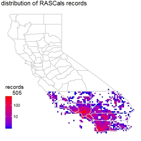
I picked colors to match those used on the California Herps map. A legend would be nice, but that is left as an excercise for the reader (i.e. if you know of an easy way to do it let me know, because I was too lazy to manually set all of the legend parameters myself).

The colors used on the map correspond to: Light Blue = E. e. croceater – Yellow-blotched Ensatina; Purple = E. e. eschscholtzii – Monterey Ensatina; Blue = E. e. klauberi – Large-blotched Ensatina; Red = E. e. oregonensis – Oregon Ensatina; Black = E. e. picta – Painted Ensatina; Orange = E. e. platensis – Sierra Nevada Ensatina; E. e. xanthoptica – Yellow-eyed Ensatina.

Overall I was pretty happy with the results, though it is interesting to note that E. e. oregonensis seems to extend somewhat further south than shown on the California Herps map, overlapping completely with the western population of E. e. xanthoptica. According to California Herps, all E. e. oregonensis occuring in California are now regarded as intergrades, so this map may reflect some outdated taxonomic practices. There are also a few interesting “out-of-bounds” records, notably several E. e. eschscholtzii in Northern California far beyond the “normal” northern limit of their range near Monterey Bay. I have no idea if these might be misidentified or whether they are true vagrants.

I decided that it would be interesting to plot the location of hybrids on the map too, given that the presence/absence of hybridization zones is an important compenent of the ring species idea. It turns out that the ScienfiticName field from HerpNET was not as clean as I was hoping. When I downloaded the entire Ensatina dataset from HerpNET and checked the constitent taxa with levels() I got this:

 [1] "Ensatina  eschscholtzi"                                                  "Ensatina ensatina xonthoptica"                                          
 [3] "Ensatina escholtzi"                                                      "Ensatina eschschlotzii eschschlotzii"                                   
 [5] "Ensatina eschscholtzi"                                                   "ENSATINA ESCHSCHOLTZI"                                                  
 [7] "Ensatina eschscholtzi croceator"                                         "Ensatina eschscholtzi eschscholtzi"                                     
 [9] "Ensatina eschscholtzi eschscholtzi x xanthopicta"                        "Ensatina eschscholtzi klauberi"                                         
[11] "Ensatina eschscholtzi oregonensis"                                       "Ensatina eschscholtzi oregonensis x xanthopicta"                        
[13] "ENSATINA ESCHSCHOLTZI OREGONESIS"                                        "Ensatina eschscholtzi picta"                                            
[15] "Ensatina eschscholtzi picta x oregonensis"                               "Ensatina eschscholtzi platensis"                                        
[17] "Ensatina eschscholtzi platensis x croceator"                             "Ensatina eschscholtzi xanthoptica"                                      
[19] "Ensatina eschscholtzii"                                                  "ENSATINA ESCHSCHOLTZII"                                                 
[21] "Ensatina eschscholtzii cf oregonensis"                                   "Ensatina eschscholtzii croceater"                                       
[23] "Ensatina eschscholtzii croceator"                                        "Ensatina eschscholtzii escholtzi"                                       
[25] "Ensatina eschscholtzii eschscholtzi"                                     "Ensatina eschscholtzii eschscholtzii"                                   
[27] "ENSATINA ESCHSCHOLTZII ESCHSCHOLTZII"                                    "Ensatina eschscholtzii eschscholtzii x Ensatina eschscholtzii klauberi" 
[29] "Ensatina eschscholtzii eschscholtzii x eschscholtzii oregonensis"        "Ensatina eschscholtzii eschscholtzii x xanthoptica"                     
[31] "Ensatina eschscholtzii klauberi"                                         "Ensatina eschscholtzii oregonensis"                                     
[33] "ENSATINA ESCHSCHOLTZII OREGONENSIS"                                      "Ensatina eschscholtzii oregonensis x Ensatina eschscholtzii xanthoptica"
[35] "Ensatina eschscholtzii oregonensis x eschscholtzii picta"                "Ensatina eschscholtzii oregonensis X picta"                             
[37] "Ensatina eschscholtzii oregonensis x platensis"                          "Ensatina eschscholtzii oregonensis x xanthoptica"                       
[39] "Ensatina eschscholtzii picta"                                            "ENSATINA ESCHSCHOLTZII PICTA"                                           
[41] "Ensatina eschscholtzii picta x oregonensis"                              "Ensatina eschscholtzii platensis"                                       
[43] "ENSATINA ESCHSCHOLTZII PLATENSIS"                                        "Ensatina eschscholtzii platensis x Ensatina eschscholtzii xanthoptica"  
[45] "Ensatina eschscholtzii ssp."                                             "Ensatina eschscholtzii xanthoptica"                                     
[47] "ENSATINA ESCHSCHOLTZII XANTHOPTICA"                                      "Ensatina eschscholzii"                                                  
[49] "Ensatina sp."

Yikes. Note that “Ensatina eschscholtzii oregonensis x Ensatina eschscholtzii xanthoptica” and “Ensatina eschscholtzii oregonensis x xanthoptica” appear as separate levels. This variable formatting is probably worth being aware of if you work on species that hybridize. Likewise, I noticed that my original queries also returned hybrids when the complete parent taxon name was included in taxonomic identification of the specimen. Thus an individual identified as “Ensatina eschscholtzii oregonensis x Ensatina eschscholtzii xanthoptica” would appear in queries for “Ensatina eschscholtzii oregonensis” and “Ensatina eschscholtzii xanthoptica” but a hybrid identified as “Ensatina eschscholtzii oregonensis x xanthoptica” would only appear in the former.

I began cleaning this up using gsub() to standardize the formatting when eventually my wife came in the room and asked “have you been working on that salamander thing ALL day?” At which point I realized I should probably get back to my own dissertation work.

Fun stuff though. Thanks Vijay!

library(rvertnet)
library(ggplot2)
library(maps)

YBE<-vertoccurrence(t="Ensatina eschscholtzii croceater",grp="herp")
YBE2<-subset(YBE,Latitude !=0 & Longitude != 0)
ME<-vertoccurrence(t="Ensatina eschscholtzii eschscholtzii",grp="herp")
ME2<-subset(ME,Latitude !=0 & Longitude != 0)
LBE<-vertoccurrence(t="Ensatina eschscholtzii klauberi",grp="herp")
LBE2<-subset(LBE,Latitude !=0 & Longitude != 0)
OE<-vertoccurrence(t="Ensatina eschscholtzii oregonensis",grp="herp")
OE2<-subset(OE,Latitude !=0 & Longitude != 0)
PE<-vertoccurrence(t="Ensatina eschscholtzii picta",grp="herp")
PE2<-subset(PE,Latitude !=0 & Longitude != 0)
SNE<-vertoccurrence(t="Ensatina eschscholtzii platensis",grp="herp")
SNE2<-subset(SNE,Latitude !=0 & Longitude != 0)
YE<-vertoccurrence(t="Ensatina eschscholtzii xanthoptica",grp="herp")
YE2<-subset(YE,Latitude !=0 & Longitude != 0)

all_states<-map_data("state")
states <- subset(all_states, region %in% c("california") )
emap <- ggplot()
emap <- emap + geom_polygon( data=states, aes(x=long, y=lat, group = group),colour="white", fill="grey90" )+theme_bw()

emap +
geom_jitter(data = YBE2,aes(Longitude, Latitude), alpha=0.3, color = "light blue") +
opts(title = "Ensatina subspecies")+
geom_jitter(data = ME2,aes(Longitude, Latitude), alpha=0.3, color = "purple")+
geom_jitter(data = LBE2, aes(Longitude, Latitude), alpha=0.3, color = "blue")+
geom_jitter(data = OE2,aes(Longitude, Latitude), alpha=0.3, color = "red")+
geom_jitter(data = PE2,aes(Longitude, Latitude), alpha=0.3, color = "black")+
geom_jitter(data = SNE2, aes(Longitude, Latitude), alpha=0.3, color = "orange")+
geom_jitter(data = YE2, aes(Longitude, Latitude), alpha=0.3, color = "yellow")+
xlim(c(-125,-113))+ylim(c(30,43))

Blue Jay and Scrub Jay : Using rvertnet to check the distributions in R

30 Jul

As part of my Google Summer of Code, I am also working on another package for R called rvertnet. This package is a wrapper in R for VertNet websites. Vertnet is a vertebrate distributed database network consisting of FishNet2MaNISHerpNET, and ORNIS. Out of that currently Fishnet, HerpNET and ORNIS have their v2 portals serving data. rvertnet has functions now to access this data and import them into R data frames.

Some of my lab mates faced a difficulty in downloading data for Scrub Jay (Aphelocoma spp. ) due to large number of records (220k+) on ORNIS, so decided to try using rvertnet package which was still in development that time. The package really helpe and got the results quickly. So while ecploring that data I came up with this case study.

So here to get data for Blue Jay (Cyanocitta cristata) which is distributed in eastern USA, we use vertoccurrence function and specify taxon we are looking for as Blue Jay with t=”Cyanocitta cristata” and we need to specify this is bird species with grp=”bird” since currently we have to access the data form three different websites of VertNet for Fishes, Birds and Herps(Reptiles and Amphibians). This fetches us all the records for Blue Jay. Now we want to get discard the records without Latitude and Longitude values so we use subset function on the data with Latitude !=0 & Longitude != 0. This gives us all geocoded records for Blue jay which then map using maps and ggplot packages like we did in earlier post.

library(rvertnet)
bluej1=vertoccurrence(t="Cyanocitta cristata",grp="bird")
bluej2=subset(bluej1,Latitude !=0 & Longitude != 0)

library(maps)
library(ggplot2)
world  = map_data("world")
ggplot(world, aes(long, lat)) +
  geom_polygon(aes(group = group), fill = "white",
               color = "gray40", size = .2) +
  geom_jitter(data = bluej2,
              aes(Longitude, Latitude), alpha=0.6, size = 4,
              color = "red") +
                opts(title = "Cyanocitta cristata (Blue Jay)")

The final output of the code snippet is as following.

Now let us put Blue Jay and Scrub Jay side by side on the map to see how they are distributed in North America.  This is same as the earlier code except that we get data for both Jays and while plotting we use additional geom_jitters for the other Jay with a different color to distinguish the two. Also not the reduction in the size from 4 to 1 in order to make the points clearly visible

library(rvertnet)
bluej1=vertoccurrence(t="Cyanocitta cristata",grp="bird")
bluej2=subset(bluej1,Latitude !=0 & Longitude != 0)
scrubj1=vertoccurrence(t="Aphelocoma",grp="bird")
scrubj2=subset(scrubj1,Latitude !=0 & Longitude != 0)

library(maps)
library(ggplot2)
world = map_data("world")
ggplot(world, aes(long, lat)) +
  geom_polygon(aes(group = group), fill = "white", color = "gray40",
               size = .2) +
  geom_jitter(data = bluej2,
              aes(Longitude, Latitude), alpha=0.6, size = 1,
              color = "blue") +
                opts(title = "Blue Jay and Scrub Jay") +
  geom_jitter(data = scrubj2,
              aes(Longitude, Latitude), alpha=0.6, size = 1,
              color = "brown")

The final output of the code snippet is as following.

Map biodiversity records with rgbif, maps and ggplot2 packages in R

9 Jul

Global Biodiversity Information Facility or GBIF is an international consortium working towards making Biodiversity information available through single portal to everyone.  GBIF with its partners are working towards mobilizing data, developing data and metadata standards, developing distributed database system and making the data accessible through APIs. At this point this largest single window data source covering wide spectrum of taxa and geographic range.

rgbif is a package in R to download the data from GBIF data portal using its API. Once the data is available as data frame in R, we can use several functions and packages to analyse and visualize it. [ Cran, rOpenSci, my work ]

Here first we use occurrencelist function to download 1000 records (maxresults = 1000) for “Danaus plexipus”  (sciname = ‘Danaus plexippus’) which is Monarch Butterfly. We specify that we want records that have been geo-coded (coordinatestatus=TRUE), we want it to be stored in data frame (latlongdf=TRUE) and we want to remove any records that have zeros in Latitude and Longitude values (removeZeros = TRUE). This command will result in a data frame dan_ple with monarch occurrence records.

Now we use map_data function form maps package to get world map. Use ggplot function form ggplot2 package to plot the world map as polygon layer. On top of that we plot the Monarch butterfly occurrence points using decimalLatitude and decimalLongitude columns in red color. and specify the title of the map.

library(rgbif)
dan_ple=occurrencelist(sciname = 'Danaus plexippus', 
                       coordinatestatus = TRUE, maxresults = 1000, 
                       latlongdf = TRUE, removeZeros = TRUE)
library(maps)
library(ggplot2)
world = map_data("world")
ggplot(world, aes(long, lat)) +
geom_polygon(aes(group = group), fill = "white", 
              color = "gray40", size = .2) +
geom_jitter(data = dan_ple,
aes(decimalLongitude, decimalLatitude), alpha=0.6, 
             size = 4, color = "red") +
opts(title = "Danaus plexippus")

The final output of the code snippet is as following.

Map of Danaus plexippus

More maps using other packages to come soon.